3.4.4 HARDNESS (ASTM D 2240)

3.4.4 HARDNESS (ASTM D 2240):

SHORE – A:

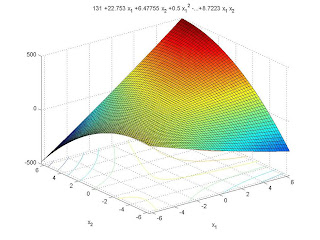
The Shore – A Hardness test was performed as per the procedure explained in the chapter 2 and the results were tabulated as shown in table 3.15. From the results, regression analysis had been performed to get the regression equation, which is shown in the table 3.16. Then using the equation contour plots and response surfaces are generated which are shown in fig 3.21 and 3.22. The desired values of

Shore – A Hardness can be obtained at any combination within the optimized region as indicated in the contour plot. The value of X1 varies from 68 – 82 and X2 varies from 10 – 20 in the optimum region.

SHORE – D:

The Shore – A Hardness test was performed as per the procedure explained in the chapter 2 and the results were tabulated as shown in table 3.15. From the results, regression analysis had been performed to get the regression equation, which is shown in the table 3.17. Then using the equation contour plots and response surfaces are generated which are shown in fig 3.23 and 3.24. The desired values of

Shore – D Hardness can be obtained at any combination within the optimized region as indicated in the contour plot. The value of X1 varies from 55 - 67 and X2 17 - 25 varies from in the optimum region.

Table 3.15 Results of Shore – A and Shore – D Hardness tests for CaCO₃ – HDPE system:

TRIAL	X1	X2	SHORE – A HARDNESS	SHORE – D HARDNESS
1	60	5	76	54.3
2	60	25	79.0	56.0
3	80	5	81.0	58.3
4	80	25	78.3	56.3
5	56	15	78.3	59.0
6	84	15	80.3	58.0
7	70	1	78.0	57.3
8	70	29	80.6	57.3
9	70	15	81.0	57.6
10	70	15	81.0	57.6
11	70	15	81.0	57.6

Table 3.16 Estimated Regression Coefficients for Hardness- Shore A

Term	Coef	SE Coef	T	P
Constant	81.0095	0.4285	189.037	0.000
X1	0.9003	0.2638	3.413	0.019
X2	0.5119	0.2638	1.940	0.110
X1*X1	-1.0388	0.3166	-3.281	0.022
X2*X2	-1.0388	0.3166	-3.281	0.022
X1*X2	-1.4175	0.3712	-3.819	0.012

S = 0.7424 R-Sq = 90.3% R-Sq (adj) = 80.7%

The regression equation is

Y = 81.0095 +0.9003X₁ +0.5119X₂ -1.0388X₁² -1.0388X₂² -1.4175X₁ X₂.

Table 3.17 Estimated Regression Coefficients for Hardness- Shore D

Term	Coef	SE Coef	T	P
Constant	57.6223	0.8001	72.015	0.000
X1	0.3699	0.4925	0.751	0.486
X2	-0.0417	0.4925	-0.085	0.936
X1*X1	0.0210	0.5912	0.035	0.973
X2*X2	-0.5760	0.5912	-0.974	0.375
X1*X2	-0.9175	0.6930	-1.324	0.243

S = 1.386 R-Sq = 40.3% R-Sq (adj) = 0.0%

The regression equation is

Y = 57.6223 +0.3699X₁ -0.0417X₂ +0.0210X₁² -0.576X₂² -0.9175X₁ X₂.

Fig. 3.21 Contour Plot of Hardness – Shore A vs. X1, X2

Fig. 3.22 Response surface of Hardness – Shore A vs. X1, X2

Fig. 3.23 Contour plot of Hardness – Shore D vs. X1, X2

Fig. 3.24 Response surface of Hardness – Shore D vs. X1, X2

OVERLAYING OF CONTOUR PLOTS:

The individual contour plots were generated for each of the property and then simultaneous optimization of properties were carried out by overlaying the individual plots to obtain the overlaid contour plots.

The desired values of all these properties can be obtained at any given combination within the optimized region indicated by the white coloured region in the fig.3.20. The values of both X1 and X2 vary over a wide range in the optimized region.

The desired values of all these properties can be obtained at any given combination within the optimized region indicated by the white coloured region in the fig.3.13. The value of X1 varies from 77 – 80 and X2 varies from 5 – 17 in the optimized region.

Fig. 3.20 Overlaid Contour plot of Tensile Properties

Fig. 3.13 Overlaid contour Plot of Flexural Properties

3.4.3 TENSILE PROPERTIES (ASTM D-638)

3.4.3 TENSILE PROPERTIES (ASTM D-638):

The tensile strength test was performed as per the procedure explained in the chapter 2 and the results were tabulated as shown in table 3.11. The properties that were evaluated as a part of tensile strength test are tensile strength at break load, percentage elongation at break load and Youngs modulus. From the results, regression analysis had been performed to get the regression equations, which are shown in the tables 3.12, 3.13, 3.14. Then using the equations contour plots and response surfaces were generated for each of them as shown in the figures 3.14 – 3.19.

Table 3.11 Results of Tensile Properties for CaCO₃ – HDPE system

Trial no.	X1	X2	Youngs modulus (kg/cm2 )	Tensile strength @ break load (kg/cm2 )	Percentage elongation @ break load
1.	60	5	1214	104	80.2
2.	60	25	1157	119	66.5
3.	80	5	1337	159	90.5
4.	80	25	1205	176	174
5.	56	15	840	92.5	66.4
6.	84	15	1113	142	193
7.	70	1	1318	137	52
8.	70	29	1135	151	87
9.	70	15	1297	131	68.6
10.	70	15	1297	131	68.6
11.	70	15	1297	131	68.6

Table 3.12 Estimated Regression Coefficients for Tensile Strength @ break load

Term	Coef	SE Coef	T	P
Constant	130.882	5.054	25.895	0.000
X1	22.891	3.111	7.358	0.001
X2	6.515	3.111	2.094	0.090
X1*X1	-4.690	3.735	-1.256	0.265
X2*X2	8.958	3.735	2.399	0.062
X1*X2	0.500	4.378	0.114	0.914

S = 89.52 R-Sq = 80.4% R-Sq (adj) = 60.8%

The regression equation is

Y = 130.882+ 22.891X₁ +6.515X₂ -4.69X₁² +8.958X₂² +0.5X₁ X₂.

Table 3.13 Estimated Regression Coefficients for Tensile Strength Youngs Modulus

Term	Coef	SE Coef	T	P
Constant	1295.26	51.68	25.064	0.000
X1	69.85	31.81	2.196	0.080
X2	-56.21	31.81	-1.767	0.137
X1*X1	-129.30	38.18	-3.386	0.020
X2*X2	-1.74	38.18	-0.046	0.965
X1*X2	-18.75	44.76	-0.419	0.693

S = 89.52 R-Sq = 80.4% R-Sq (adj) = 60.8%

The regression equation is

Y = 1295.26+ 69.85X₁ -56.21X₂ -129.3X₁² -1.74X₂² -18.75X₁ X₂.

Table 3.14 Estimated Regression Coefficients for Percentage Elongation

Term	Coef	SE Coef	T	P
Constant	68.566	6.073	11.290	0
X1	37.253	3.738	9.965	0
X2	15	3.738	4.012	0.01
X1*X1	31.846	4.488	7.096	0.001
X2*X2	1.131	4.488	0.252	0.811
X1*X2	24.3	5.260	4.619	0.006

S = 10.52 R-Sq = 97.41% R-Sq (adj) = 94.9%

The regression equation is

Y = 68.566+ 37.253X₁ +15X₂ +31.846X₁² +1.131X₂² +24.3X₁ X₂.

Fig. 3.14 Contour Plot of tensile strength at break load vs. X2, X1

Fig. 3.15 Response surface of tensile strength at break load vs. X2, X1

Fig. 3.16 Plot of Youngs Modulus vs. X1

Fig. 3.17 Response surface of Youngs Modulus vs. X2, X1

Fig. 3.18 Contour plot of Percentage Elongation vs. X2, X1

Fig. 3.19 Response surface of Percentage Elongation vs. X2, X1